Finding Eigenvalues

How these little guys actually get computed

In AI, eigenvectors and eigenvalues are everywhere. You see them in places like principal component analysis¹, RNN stability analysis², and optimization analysis³. For a square matrix A, an eigenvector is a vector v, along with a corresponding scalar λ, the eigenvalue, such that:

\(Av = \lambda v\)

The key idea is that applying the linear transformation A to the eigenvector v scales the vector’s magnitude, but otherwise leaves it untransformed. I recently dug into how eigenvectors and eigenvalues get computed in practice, and I wanted to share it, because it was fairly unintuitive, and actually kind of cool.

First, it’s worth sharing how I learned to compute eigenvalues back in school, since you might have seen this in a linear algebra class somewhere. Note that:

\(\begin{align} Av &= \lambda v \\ Av - \lambda v &= 0 \\ Av - \lambda I v &= 0 \\ (A - \lambda I) v &= 0 \end{align}\)

Assuming v is a non-zero eigenvector, this then implies that

\(\textrm{det}(A - \lambda I)=0\)

For an n×n matrix A, this determinant expression translates into a n^th order polynomial of λ. The roots of this equation are the eigenvalues of A. For a given eigenvalue λ_i of A, you can find the corresponding eigenvector by plugging this into the equation and solving for v_i:

\((A-\lambda_i I)v_i = 0\)

That’s all great, but that doesn’t tell you how to actually compute the roots of the polynomial. I did some digging and discovered that standard root-finding algorithms like Matlab’s⁴ find the roots by finding eigenvalues of the polynomial’s companion matrix⁵, so this seems circular:

1. To find the eigenvalues of a matrix, just find the roots of a corresponding polynomial.

2. To find the roots of a polynomial, just find the eigenvalues of a corresponding matrix.

I decided to go down the rabbit hole and get to the bottom of this. Here’s a quick summary of how modern libraries actually find eigenvalues.

Triangular Matrices

Note that if you have an upper-triangular matrix, like:

\(\begin{bmatrix} a_{11} & a_{12} & \cdots & a_{1n} \\ 0 & a_{22} & \cdots & a_{2n} \\ \vdots & \vdots & \ddots & \vdots \\ 0 & 0 & \cdots & a_{nn} \end{bmatrix},\)

then the eigenvalues are just the diagonal entries of the matrix, since:

\(\textrm{det}(A - \lambda I)= (a_{11} - \lambda)(a_{22} - \lambda)\cdots(a_{nn} -\lambda)\)

This is key, because the general algorithm for finding eigenvalues transforms the matrix into a triangular matrix with the same eigenvalues. Once you’ve done this, your done, since you can just read the diagonal entries as the eigenvalues.

Matrix Similarity

Two matrices A and B are similar⁶ if there exists an invertible matrix P, such that

\(B = P^{-1}AP\)

A key property of similar matrices is that they have the same eigenvalues. So the basic idea of finding eigenvalues for A is to find a similar matrix to A that’s also upper triangular.

Schur decomposition

For any square matrix A, there exists an orthogonal matrix Q_* and an upper triangular matrix H such that

\(A = Q_*^{-1}HQ_*\)

Q_* being orthogonal is just a fancy way of saying:

\(Q_*^TQ_* = I\)

Since H is upper triangular, once you have the Schur decomposition, the eigenvalues are just the diagonal entries of H.

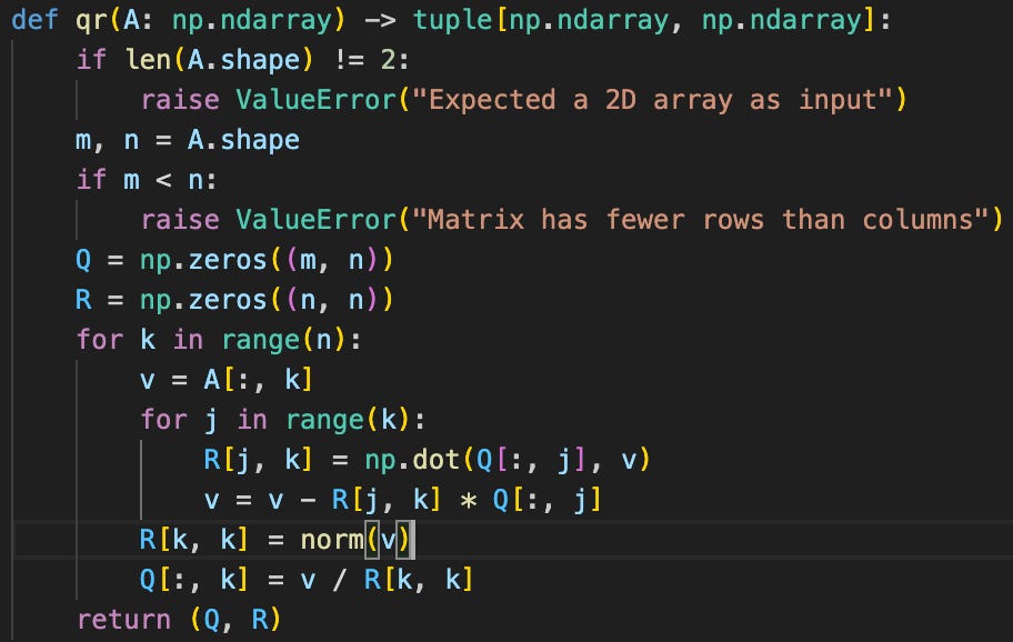
The tricky part is computing the Schur decomposition. To get that, modern eigenvalue solvers use a simpler matrix decomposition: the QR decomposition⁷. The QR decomposition is just a breakdown of A into an orthogonal matrix Q and an upper triangular matrix R:

\(A = QR\)

QR decomposition is straightforward. A simple implementation using the Gram-Schmidt⁸ process is shown here:

A more popular implementation uses Householder reflections⁹. Householder reflections are a bit less straightforward than Gram-Schmidt, but they are the de facto implementation, because they have better numerical stability.

There’s a neat property of QR decomposition that lets you use it to find the Schur decomposition. First, note that for an orthogonal Q:

\(\begin{align} Q^TAQ &= Q^T(QR)Q \\ &= (Q^TQ)RQ \\ &= RQ \\ \end{align}\)

Q^TAQ is a similar matrix to A. If you set:

\(\begin{align} A_0 &= A \\ Q_i, R_i &= \textrm{qr-decomp}(A_i) \\ A_{i+1} &= R_iQ_i \\ \end{align}\)

you then get a sequence (A₀, A₁, …) of similar matrices to A. This sequence has the nifty property¹⁰ that

\(\lim_{k \to \infty} A_k = Q_*AQ_*^T=H\)

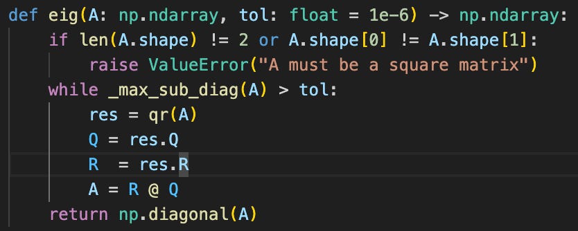
where Q* is the orthogonal matrix from the Schur decomposition, and H is the upper-triangular matrix Schur matrix. This gives you your eigenvalues, from it’s diagonals. This means you can use code like this to find the eigenvalues:

This is not too different than what production eigenvalue solvers do. There are a couple of key changes they make, for better performance, however:

1. Before the first step, they transform A into an upper Hessenberg¹¹ form. This is a one-time transformation that costs O( n³ ) time, but it then reduces the time of each QR step in the loop from O( n³ ) to O( n² ).

2. At each step, they perform a Wilkinson shift¹². This is a transformation to the matrix that makes the overall loop go from having linear convergence to quadratic convergence, for the general case, and cubic convergence when A is symmetric.

1. Pearson, K. (1901). LIII. On lines and planes of closest fit to systems of points in space . The London, Edinburgh, and Dublin Philosophical Magazine and Journal of Science, 2(11), 559–572. https://doi.org/10.1080/14786440109462720

2. Panda, Priyadarshini, Efstathia Soufleri, and Kaushik Roy. "Evaluating the Stability of Recurrent Neural Models during Training with Eigenvalue Spectra Analysis." 2019 International Joint Conference on Neural Networks (IJCNN). IEEE, 2019.

3. Ghorbani, B., Krishnan, S. &amp; Xiao, Y.. (2019). An Investigation into Neural Net Optimization via Hessian Eigenvalue Density. <i>Proceedings of the 36th International Conference on Machine Learning</i>, in <i>Proceedings of Machine Learning Research</i> 97:2232-2241 Available from https://proceedings.mlr.press/v97/ghorbani19b.html.

4. MathWorks. “Roots – Polynomial Roots – MATLAB.” MATLAB Documentation, MathWorks, www.mathworks.com/help/matlab/ref/roots.html. Accessed 26 May 2025.

5. “Companion Matrix.” Wikipedia, Wikimedia Foundation, https://en.wikipedia.org/wiki/Companion_matrix. Accessed 26 May 2025.

6. “Matrix Similarity.” Wikipedia, Wikimedia Foundation, https://en.wikipedia.org/wiki/Matrix_similarity. Accessed 26 May 2025.

7. “QR Decomposition.” Wikipedia, Wikimedia Foundation, 9 May 2025, https://en.wikipedia.org/wiki/QR_decomposition. Accessed 26 May 2025.

8. “Gram–Schmidt Process.” Wikipedia, Wikimedia Foundation, https://en.wikipedia.org/wiki/Gram%E2%80%93Schmidt_process. Accessed 26 May 2025.

9. “Householder Transformation.” Wikipedia, Wikimedia Foundation, https://en.wikipedia.org/wiki/Householder_transformation. Accessed 26 May 2025.

10. Falk, Richard S. “Convergence of the QR Algorithm.” Math 574 Lecture Notes, Rutgers U, 2004, pp. 32‑33. sites.math.rutgers.edu

11. “Hessenberg Matrix.” Wikipedia, Wikimedia Foundation, https://en.wikipedia.org/wiki/Hessenberg_matrix. Accessed 26 May 2025.

12. Yang, Ming-Hsuan. “Lecture 17.” EECS 275: Matrix Computation, University of California, Merced, https://faculty.ucmerced.edu/mhyang/course/eecs275/lectures/lecture17.pdf. Accessed 26 May 2025.