Entropy explained

Disorderly conduct

Entropy is a concept that comes up repeatedly in AI. After recently watching a great video on the history of information theory, I thought it would be cool to make a short explainer on entropy, both generally, and specific to AI/ML.

The idea of entropy was originally created in physics, defined as a measure of disorder and irreversibility in thermodynamic systems. Intuitively, entropy quantifies how dispersed or random the energy in a system is. The Second Law of Thermodynamics states that in an isolated system, one with no energy exchange with the environment, entropy tends to increase or remain constant. In other words, natural processes lead to greater disorder over time¹. A classic example is heat flowing from a hot object to a cold one: the energy spreads out and becomes less available to do work, increasing the overall entropy of the combined system.

In statistical mechanics, if a system can be in microstate i with probability p_i​, then the Gibbs entropy is:

\(S = -k_B \sum_i p_i \ln p_i ,\)

where k_B is the Boltzmann constant². Here a microstate is the specific arrangement of the particles in the system: their positions and momentums. This Gibbs entropy formula is deeply connected to the concept of information entropy.

Entropy in information theory

In 1948, Claude Shannon introduced entropy in the context of information theory to quantify uncertainty in a data source³. Information entropy measures the average information content or “surprise” of a random variable. For a discrete random variable X with possible outcomes {x₀, x₁, …} having corresponding probability {p₀, p₁, …}. The entropy H is defined as:

\(H(p) = - \sum_i p_i \log_2 p_i\)

To get some intuition around this formula, consider the entropy of a coin toss, where the probability of flipping heads varies from 0 to 1:

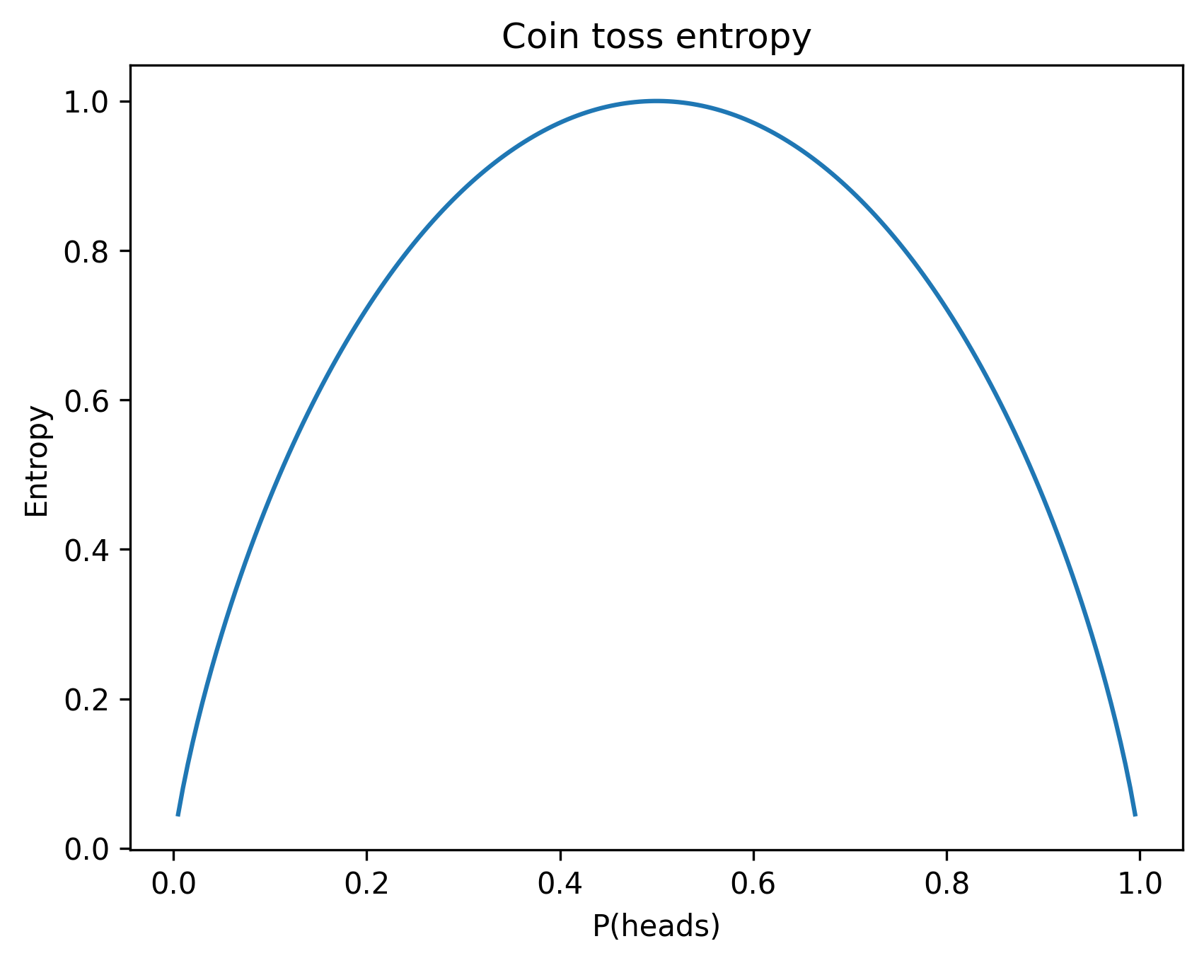
Note that the entropy is greatest when heads and tails are equally likely. The entropy converges to zero whenever there is no randomness to the coin toss. Intuitively, there are more “surprises” in flipping an fair coin, than when flipping an unfair one.

Note that entropy provides a lower bound for the average number of bits required to transmit or store a sequence of events drawn from a probability distribution. Also, you can find an encoding that gets arbitrarily close to this lower bound. Consider the case where P(heads) = 2/3 and P(tails) = 1/3. The entropy in this case is roughly 0.918. If you encode pairs of heads/tails sub-sequences using this encoding:

• heads, heads => 0

• heads, tails => 10

• tails, heads => 110

• tails, tails => 111

then average number of bits required to encode two symbols is 1.889, and the average number of bits per symbol is 0.944. You can reduce this number closer to the lower bound by increasing the size of the subsequence used in the encoding.

A related idea to entropy is cross entropy⁴. Let’s say the true probability distribution is p, but your estimate of the distribution is q. Then the cross entropy (also written with H) is defined as:

\(H(p, q) = -\sum_i p_i \log_2 q_i\)

In information theory, cross entropy provides a lower bound for the average number of bits required to transmit or store a sequence of events drawn from a probability distribution p when you estimate the distribution is q. H(q, p) will always be greater than or equal to H(p), so there’s a cost to bad estimation. The difference between H(q, p) and H(p) is called the Kullback–Leibler (KL) divergence:

\(\begin{eqnarray} D_{KL}(p || q) &= H(p, q) - H(p) \\ &= \sum_i p_i \log_2 \frac{p_i}{q_i} \end{eqnarray}\)

Entropy in machine learning

In machine learning, cross entropy is commonly used as a loss function for classification problems⁵. In a classification problem with c classes, each output y is a vector of length c, where y_i is 1 when the label belongs to class i, and 0 for all other entries. For example, an output might be y = (0, 0, 1, 0). An estimate of the output ŷ might be something like (0.1, 0.05, 0.8, 0.05). The cross-entropy loss function is:

\(l(y, \hat{y}) = -\sum_{i} y_i \log_2 \hat{y}_i\)

This is the same as the cross-entropy function above replacing (p, q) with (y, ŷ). Just like in the information theory case, this function is minimized when y = ŷ.

To see an example of what this loss function looks like, let y = (1, 0), and ŷ = (a, 1-a), for 0 < a ≤ 1:

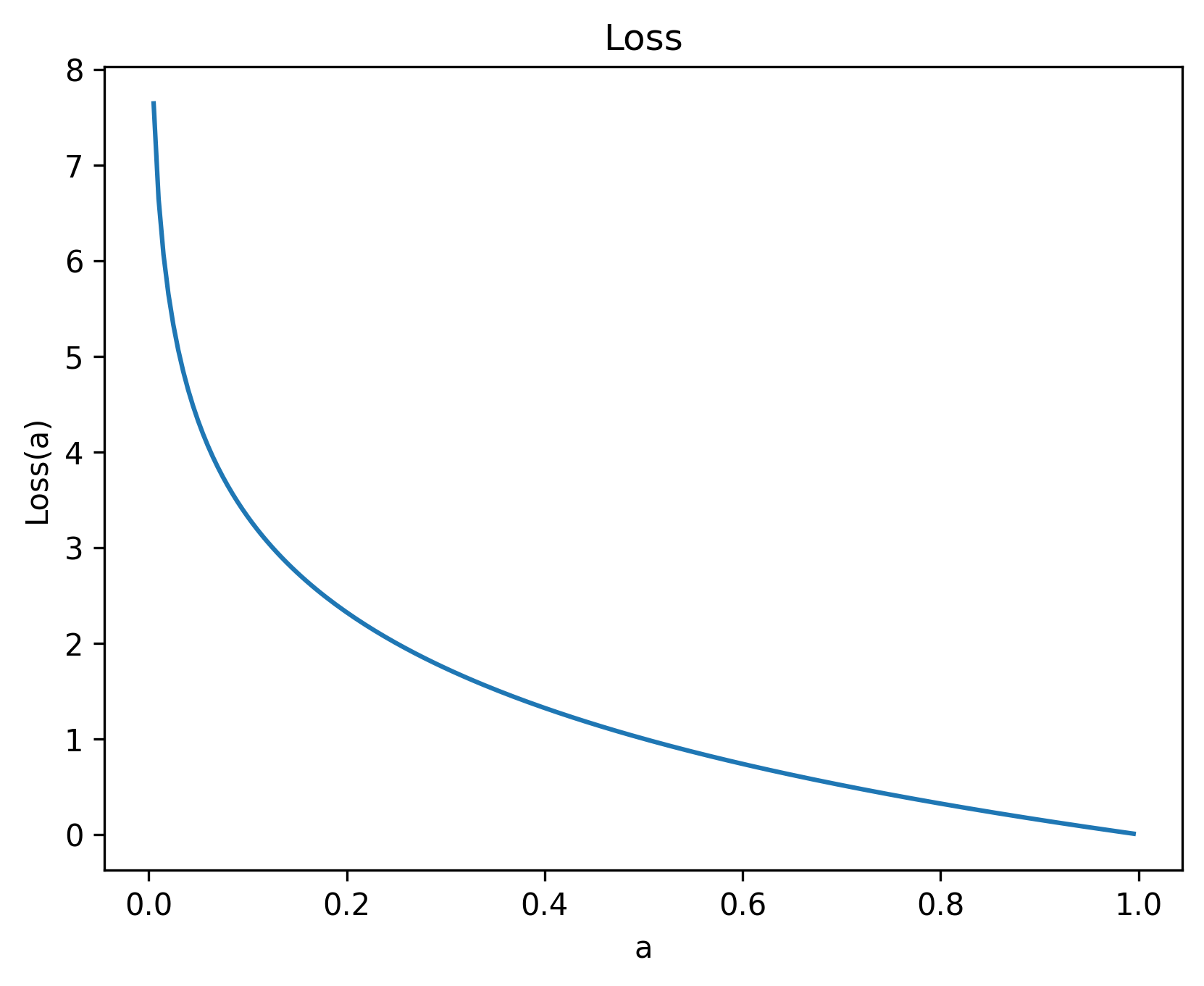
The loss equals zero when a =1.

There are other uses of entropy in machine learning, in addition to cross-entropy loss. KL divergence often appears in scenarios where you explicitly want to push one probability distribution toward another. For example, in variational inference and variational autoencoders (VAEs), the training objective includes a KL divergence term to make an approximate posterior close to a prior⁶. In reinforcement learning, algorithms like Trust Region Policy Optimization⁷ and Proximal Policy Optimization⁸ constrain or penalize the KL divergence between the new and old policy to ensure gradual updates.

1. Urone, Paul Peter, and Roger Hinrichs. "12.3 Second Law of Thermodynamics: Entropy." Physics, OpenStax, 26 Mar. 2020, https://openstax.org/books/physics/pages/12-3-second-law-of-thermodynamics-entropy.

2. "Entropy (Statistical Thermodynamics)." Wikipedia, Wikimedia Foundation, https://en.wikipedia.org/wiki/Entropy_(statistical_thermodynamics). Accessed 29 May 2025.

3. Shannon, Claude E. "A Mathematical Theory of Communication." Bell System Technical Journal, vol. 27, no. 3, 1948, pp. 379–423, and no. 4, pp. 623–656.

4. "Cross-Entropy." Wikipedia: The Free Encyclopedia, Wikimedia Foundation, https://en.wikipedia.org/wiki/Cross-entropy. Accessed 29 May 2025.

5. Zhang, Aston, et al. “4.1 Softmax Regression.” Dive into Deep Learning, https://d2l.ai/chapter_linear-classification/softmax-regression.html. Accessed 29 May 2025.

6. Kingma, Diederik P., and Max Welling. "Auto-Encoding Variational Bayes." arXiv, 20 Dec. 2013, https://arxiv.org/abs/1312.6114.

7. Schulman, John, Sergey Levine, Pieter Abbeel, Michael Jordan, and Philipp Moritz. "Trust Region Policy Optimization." Proceedings of the 32nd International Conference on Machine Learning, vol. 37, 2015, pp. 1889–1897. Proceedings of Machine Learning Research, https://proceedings.mlr.press/v37/schulman15.html.

8. Schulman, John, et al. "Proximal Policy Optimization Algorithms." arXiv, 28 Aug. 2017, https://arxiv.org/abs/1707.06347.